By Samadrita Karmakar
Introduction
Ever heard of the Butterfly Effect?
If you have not heard about it, let me give you an idea. It is based on the concept that even small changes in a system, somewhere now (initial condition), may give rise to big events in the future. Say if the system is the atmosphere all around you, then the small changes in air flow due to a butterfly flapping its wings miles away, from where you are reading this blog, gives rise to a tornado reaching near you in the next few weeks.
Mathematics and Chaos?
The nature surrounding us does not know mathematics. But as humans and our incessant need to find patterns in the universe, we developed this tool and it is an quite effective one. Interestingly even this tool developed by humans show Chaotic behaviour just like nature. Consider the below equation, known as logistic map of second order.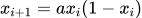
Look at the two figures below. Figure 1 has  which results in the solution stabilizing to
  . The other has figure, Figure 2 has
  solution which changes a lot even to a small change in the starting value of
  on the left side. This is an example of the final value changing drastically to the starting value, also known as the initial condition.
Lorenz and Deterministic Chaos.
In 1961, Edward Norton Lorenz, was working at the MIT Department of Meteorology. He was trying to solve an atmospheric model on a Royal McBee LGP-30. LGP-30 was a simple computer. He wanted to re-look at some of his earlier results and to save time, he decided to restart the computation after already running it for some time. He would save the last set of results by printing out the last solution on a piece of paper and then using these to perform the next set of computations.
On performing the computations, he was surprised. The computer would end up returning completely different results from the earlier ones. The reason for this variation was due to the fact that even if the computer had a 6 digit precision, the printer had one of 3. An output such as,  would be printed as
  . This rounding-off of numbers caused the divergence in results. The discovery, made Lorenz an early pioneer in a new area of research. It is now known as Deterministic Chaos or simply, Chaos.
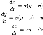
Lorenz in 1963 with the help of Ellen Fetter came up with a very simplified model of atmospheric convection that later on came to be known as Lorenz system. I do not need you to understand the meaning of the equations. All I wish to do is encourage you to appreciate is its implication. Do note how the three states (here, particles) started off from pretty much the same place and are almost indistinguishable from one another but end up following completely different trajectories.
Deterministic Chaos in Weather Prediction.
Edward Norton Lorenz was a meteorologist, and he was working on atmospheric models. So it is quite obvious that deterministic chaos would have important implications in weather prediction. Meteorologists try to take into account multiple initial conditions. But the number of options of such initial conditions could be huge.There are ways not only to choose from the large options of initial conditions but also one has to choose on how to conduct such simulations and what kind of interpretations can be made on them. If you wish to have a better idea of how such simulations are conducted, I recommend you to read my colleague Alexander Moriggl's blog here.
References:
If you are interested in knowing which article and videos I used as references for writing this blog, here are a few of them below:- Wikipedia: Chaos Theory
- YouTube: Chaos: The Science of the Butterfly Effect
- YouTube: The Logistic Map
- Wikipedia: Edward Norton Lorenz
- Wikipedia: Lorenz System
Appendix
I used Julia Language to create the animations. If you wish to try them out yourself, I am pasting them below:Logistic Map:
using Plots
Plots.pyplot()

#Use "logisticMap(:stable)" to generate stable plot and "logisticMap(::unstable)" to create unstable plots
function logisticMap(type::Symbol=:stable)
    points = 100
    x_start = LinRange(.2, 0.9, points)
    if (type == :stable)
        a = 2.5
        outputHeader = "stable"
    elseif (type == :unstable)
        a = 4.0
        outputHeader = "unstable"
    else
        error("unknown type of system: $type")
    end
    x = zeros(points)
    anim = @animate for x0 ∈ x_start
        x[1] = x0
        for i ∈ 2:points
         x[i] = a*x[i-1]*(1.0-x[i-1])
        end
        plt = plot(x, label = "x_0 = $x0", marker = :circle, legend=:topright)
        xlabel!("i")
        ylabel!("x")
        ylims!(0.0, 1.0)
    end
    gif(anim, "$(outputHeader)Plot.gif", fps = 30)
end
Lorenz System:
using Plots, LinearAlgebra, ForwardDiff, NLsolve
Plots.pyplot()
#This is a multi-particle plot. Forward Euler has been used for time integration.
function lorenzSystemMultiPt()
    σ = 10.0
    ρ = 28.0
    β = 8.0/3

    Δt = 0.02

    t_end = 40.0
    f(V) =
        begin
        x, y, z = V
        return [σ*(y-x), x*(ρ-z)-y, x*y-β*z]
    end

    v_old = [[1.0,1, 1], [1.1,1, 1], [1.0,1.1, 1]]
    v = zeros(3, 3, Int64(t_end/Δt)+1)

    i =1
    for t ∈ 0.0:Δt:t_end
        for mtPt ∈ 1:length(v_old)
            v[mtPt,:, i] = v_old[mtPt] + Δt*f(v_old[mtPt])
            v_old[mtPt] .= v[mtPt,:, i]
        end
    i+=1
    end

    anim = Animation()

    for i ∈ 1:size(v[1,1,:])[1]
        plt1 = plot3d(v[1,1,1:i], v[1,2,1:i], v[1,3,1:i], xlabel ="x", ylabel= "y", zlabel = "z", label = "Particle 1 Path" )
        scatter!([v[1,1,i]], [v[1, 2,i]], [v[1, 3, i]], label = "Particle 1")
        for mtPt ∈ 2:length(v_old)
            plot3d!(v[mtPt,1,1:i], v[mtPt,2,1:i], v[mtPt,3,1:i],  label = "Particle $mtPt Path" )
            scatter!([v[mtPt,1,i]], [v[mtPt,2,i]], [v[mtPt,3, i]],  label = "Particle $mtPt" )
        end
        if mod(i, 5)==0
            frame(anim, plt1)
        end
    end
    gif(anim, "lorenz.gif", fps=24)
end