
The monodomain model is a simplification of the bidomain model, a system of ordinary differential equations (ODE) modeling the electric activity inside the heart tissues. The monodomain model is obtained by assuming that the electric potentials inside and outside the cells are equal. In spite of this approximation, the monodomain model is able to simulate qualitative expected properties of the time-periodic electric potential. The design of this model is subject to the choice of a specific nonlinearity in the partial differential equations aforementioned. One of the most commonly used is the so-called FitzHugh-Nagumo model, corresponding to the nonlinearity proposed in the original article [Fit61] of 1961. The system of time-evolution equations is the following:
\begin{equation} \left\{ \begin{array} {ll} \displaystyle \dot{v}_{\scriptscriptstyle \mathrm{FH}} + av_{\scriptscriptstyle \mathrm{FH}}^3+bv_{\scriptscriptstyle \mathrm{FH}}^2+cv_{\scriptscriptstyle \mathrm{FH}} +dw_{\scriptscriptstyle \mathrm{FH}} = f_v & \text{in } (0,T),\\[10pt] \displaystyle \dot{w}_{\scriptscriptstyle \mathrm{FH}} + \eta w_{\scriptscriptstyle \mathrm{FH}} + \gamma v_{\scriptscriptstyle \mathrm{FH}} = f_w & \text{in } (0,T),\\[10pt] (v_{\scriptscriptstyle \mathrm{FH}},w_{\scriptscriptstyle \mathrm{FH}})(t=0) = \mathrm{z}^{(0)} \in \mathbb{R}^2. & \end{array} \right. \label{ODEFH} \tag{$\mathrm{FH}$} \end{equation}
Note that this is a coupled system, as the state variables \(v_{\scriptscriptstyle \mathrm{FH}}\) and \(w_{\scriptscriptstyle \mathrm{FH}}\) appear dependently in the two evolution equations. The coefficients \(a\), \(b\), \(c\), \(d\), \(\eta\) and \(\gamma\) are to be adjusted in order to stick to the experimental measurements. Note also that the FitzHugh-Nagumo nonlinearity is a linear combination of modes, here the polynomial basis functions \(v\mapsto v\), \(v\mapsto v^2\), \(v\mapsto v^3\) and \(w\mapsto w\). Despite its apparent simplicity, the FitzHugh-Nagumo model is still difficult to study, from a theoretical point of view and also from a numerical point of view. However, this is the simplest form we found that translates the qualitative properties of a Van-der-Pol oscillator, a property that is reasonable to assume when we aim at modeling cardiac activity.
The mathematical expressions chosen in the standard monodomain model are due to human intuition and representation. They rely on our approximation paradigms, in the present case the linear approximation with given basis functions. Such a framework offers the possibility to reduce the model to a linear algebra problem, in order to determine the coefficients of the approximation, a task that can be achieved with a data-driven approach [BPK16]. Although linear problems can in principle be solved merely with the help of an undergraduate textbook, actually the quality of the underlying approximation is in practice limited, as Kolmogorov [Kol36] quantified the quality of convergence when the number of modes increases (this is the so-called Kolmogorov n-width barrier). Since then, many other approaches have been developed for improving data-driven approximations.
What if we choose a more general and nonlinear set of approximants? Here comes the idea of replacing the linear approximation of the FitzHugh-Nagumo model by artificial neural networks (ANNs).
Given activation functions \(\rho\), we consider the following feedforward ANN parameterized with affine mappings \(\mathbf{W} = (W_{\ell})_{1\leq \ell \leq L} \) as weights:
\begin{equation} \begin{array} {rccl} \Phi(\cdot,\mathbf{W}) : & \mathbb{R}^2 & \rightarrow & \mathbb{R}^2 \\ & \mathrm{z} = (v,w) & \mapsto & W_L(\rho (W_{L-1}(\rho(\dots \rho(W_1(\mathrm{z})))))). \end{array} \label{defNN} \tag{$\mathrm{ANN}$} \end{equation}
The differential system with the ANN above as nonlinear dynamics is given as follows:
\begin{equation} \left\{ \begin{array} {ll} \displaystyle \dot{v} + \Phi_1((v,w),\mathbf{W}) = f_v & \text{in } (0,T),\\[10pt] \displaystyle \dot{w} + \Phi_2((v,w),\mathbf{W}) = f_w & \text{in } (0,T),\\[10pt] (v,w)(t=0) = \mathrm{z}^{(0)} \in \mathbb{R}^2. & \end{array} \right. \label{ODE} \tag{$\ast$} \end{equation}
ANNs are mathematical objects miming the activity of biological neurons. Recently they have been extensively and successfully used for designing automated tools achieving tasks that prior methods were not able to address. In our case, the ANNs are rather chosen as nonlinear mathematical expressions. We select them for designing the nonlinearity of the monodomain model, for several reasons:
- Their theoretical approximation capacities
(see the Universal approximation theorem, and more recently [EPGB21]). - The purely nonlinear aspect of this type of approximants.
- Changing the nature of the approximation can potentially offer better accuracy.
In [CK21] we proposed an optimal control approach for addressing the underlying learning problem, namely choosing the weights parameterizing the neural networks: A rigorous study enabled us to derive optimality conditions, and thus adjust these weights in order to minimize a misfit function representing the distance between the data and the output of the model. The purely nonlinear nature of the problem as well as other technical difficulties, related in particular to the consideration of non-smooth activation functions, constituted a challenge. For illustrating our approach, we generated artificial data corresponding to the historical FitzHugh-Nagumo model, and trained a feedforward residual neural network such that the associated state got close to the data. The data set is made up of \(K\) pairs
\begin{equation*} \big(\mathrm{z}^{(0)}_{\mathrm{data,k}}, t\mapsto \mathrm{z}_k(t)\big)_{1\leq k \leq K} \quad \text{(input/output)} \end{equation*}
with time measure \(\mu\). The formulation of the optimal control problem is as follows:
\begin{equation} \label{pbODE} \tag{$\mathcal{P}$} \left\{ \begin{array} {l} \displaystyle \min_{\mathbf{W} \in \mathcal{W}} \quad \frac{1}{2} \sum_{k=1}^K \int_0^T |\mathrm{z}_k - \mathrm{z}_{\mathrm{data},k} |_{\mathbb{R}^2}^2 \,\mathrm{d} \mu(t) , \\[5pt] \mathrm{where}\ (\mathrm{z}_k = (v,w),\mathbf{W})\ \mathrm{satisfies}\ \eqref{ODE}\ \mathrm{with}\ \mathrm{z}^{(0)} = \mathrm{z}^{(0)}_{\mathrm{data},k}. \end{array} \right. \end{equation}
The results are presented in Figure 1.
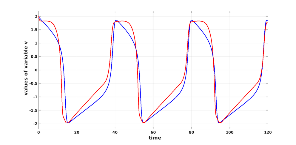
Figure 1: With the initial condition \( z(0) = (2, 0)\): The solution \(v_{\scriptscriptstyle \mathrm{FH}}\) of the FitzHugh-Nagumo model \eqref{ODEFH} in blue, and in red the solution \( v\) of \eqref{ODE} with the neural network \( \Phi\) trained by solving \eqref{pbODE}.
We conclude by mentioning that the numerical results given in Figure 1 constitute a first proof of concept of the applicability of such an approach. Improving substantially this result will certainly require the development of architectures that are more complex and more adapted to the approximation of periodic signals. Last but not least, in spite of the apparent richness of the mathematical models deployed for learning empirical phenomena, these models -- even if they are data-driven -- are not a priori supposed to translate accurately all the complexity of the cardiac electrophysiology. This is an epistemological principle: Only the comparison of mathematical models with real-world data can validate them.
The original article to this post is available here:
[CK21] Court, S., & Kunisch, K. (2021). Design of the monodomain model with artificial neural networks. ArXiv:2107.03136
Other references:
[BPK16] Brunton, S. L., Proctor, J. L., & Kutz, J. L. (2016). Discovering governing equations from data by sparse identification of nonlinear dynamical systems. Proceedings of the National Academy of Sciences, 113(15):3932–3937, 2016.
[EPGB21] Elbrächter, D., Perekrestenko, D., Grohs, P., & Bölcskei, H. (2021). Deep neural network approximation theory. IEEE Transactions on Information Theory, 67(5):2581–2623, 2021.
[Fit61] FitzHugh, F. (1961). Impulses and physiological states in theoretical models of nerve membrane. Biophysical Journal, 1(6):445–466, 1961.
[Kol36] Kolmogoroff, A. (1936). Über die beste Annäherung von Funktionen einer gegebenen Funktionenklasse. Annals of Mathematics (2), 37(1):107–110, 1936.
DOI: https://www.doi.org/10.48763/000002
This work is licensed under a Creative Commons Attribution 4.0 International License.


Written by Sébastien Court in March 2022
Assistant Professor at DiSC & Department of Mathematics
University of Innsbruck
About the author
My background are numerical simulations of fluid-structure interactions, elasticity theory, scientific computing, and optimal control theory. At the Digital Science Center, I work on the mathematical foundations of Deep Learning.
Research area
Artificial Neural Networks, Mathematical Optimization, and Dynamical Systems